After Request Filtering Why It Is Going to Filter Again

Speeding up Python Lawmaking: Fast Filtering and Wearisome Loops

List comprehensions, boolean indexing and just-in-time (JIT) compilation for up to 200x speed up.

Photo past James Donovan on Unsplash

Westhen exploring a new dataset and wanting to exercise some quick checks or calculations, ane is tempted to lazily write lawmaking without giving much thought about optimization. While this might be useful in the offset, information technology tin can easily happen that the time waiting for lawmaking execution overcomes the time that it would take taken to write everything properly.

This article shows some basic ways on how to speed up computation fourth dimension in Python. With the case of filtering data, we will hash out several approaches using pure Python, numpy, numba, pandas likewise as k-d-copse.

Fast Filtering of Datasets

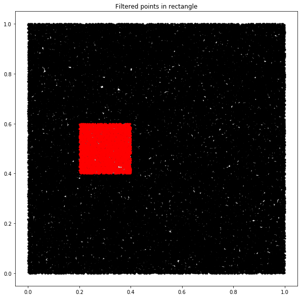
As an example chore, nosotros will tackle the problem of efficiently filtering datasets. For this, we will use points in a two-dimensional infinite, but this could exist anything in an n-dimensional space, whether this is customer information or the measurements of an experiment.

Let's suppose we would like to excerpt all the points that are in a rectangle with betwixt [0.ii, 0.4] and [0.iv, 0.6]. The naive way to do this would be to loop for each point and to check whether it fulfills this criterion. Codewise, this could look like equally follows: First, we create a function to randomly distribute points in n-dimensional space with numpy, then a function to loop over the entries. To measure computation time we utilise timeit and visualize the filtering results using matplotlib.

          Loop: 72 ms ± two.11 ms per loop (hateful ± std. dev. of vii runs, x loops each)        

As we can see, for the tested machine information technology took approx. 70 ms to excerpt the points inside a rectangle from a dataset of 100.000 points.

Note that when combining expressions you lot want to utilize a logical and (and) not a bitwise and (&). When the starting time condition is Simulated, it stops evaluating.

Although numpy is nice to interact with large n-dimensional arrays nosotros should too consider the additional overhead that we get by using numpy objects. In this detail example, we do not employ any mathematical operations where we could benefit from numpy'southward vectorization.

So at present let's criterion this loop against a pure Python implementation of the loop. Here the difference is to use a list of tuples instead of a numpy array.

          Python loop: 27.9 ms ± 638 µs per loop (mean ± std. dev. of 7 runs, ten loops each)        

The execution at present only took approx. 28 ms, so less than one-half of the previous execution time. This highlights the potential functioning decrease that could occur when using highly optimized packages for rather unproblematic tasks.

Python Functions: Listing comprehension, Map and Filter

To make a more broad comparison we will also benchmark against three built-in methods in Python: List comprehensions, Map and Filter.

• List comprehension: List comprehensions are known to perform, in general, better than for loops as they exercise not need to call the append function at each iteration.
• Map: This applies a function to all elements of an input listing.
• Filter: This returns a listing of elements for which a function returns True.

          List comprehension: 21.3 ms ± 299 µs per loop (mean ± std. dev. of 7 runs, ten loops each)
Filter:   26.8 ms ± 349 µs per loop (mean ± std. dev. of 7 runs, 10 loops each)
Map:   27 ms ± 265 µs per loop (mean ± std. dev. of 7 runs, x loops each)        

The list comprehension method is slightly faster. This is, as nosotros expected, from saving time not calling the append function. The map and filter function do not evidence a meaning speed increase compared to the pure Python loop.

Thinking about the first implementation of more than seventy ms why should one employ numpy in the first place? Ane thing nosotros tin do is to use boolean indexing. Here we perform the cheque for each criterium column-wise. We can then combine them to a boolean index and directly access the values that are within the range.

          Boolean alphabetize: 639 µs ± 28.4 µs per loop (hateful ± std. dev. of 7 runs, chiliad loops each)        

The solution using a boolean index simply takes approx. 640 µs, and then a l-fold improvement in speed compared to the fastest implementation nosotros tested so far.

Going faster: Numba

Can we even push this further? Yes, nosotros tin can. One way is to use Numba:

Numba translates Python functions to optimized car code at runtime using the industry-standard LLVM compiler library. Numba-compiled numerical algorithms in Python tin approach the speeds of C or FORTRAN.

The implementation of numba is quite piece of cake if i uses numpy and is particularly performant if the code has a lot of loops. If the functions are correctly fix, i.eastward. using loops and bones numpy functions, a elementary addition of the @njit decorator will flag the part to be compiled in numba and will be rewarded with an increment in speed. Feel gratis to bank check out numbas documentation to learn about the details in setting up numba-compatible functions.

Note that we are using the about recent version of Numba (0.45) that introduced the typed list. Additionally, note that we are executing the functions in one case before timing to not business relationship for compilation time. Now let's run into how the functions perform when being compiled with Numba:

          Boolean alphabetize with numba: 341 µs ± 8.97 µs per loop (mean ± std. dev. of 7 runs, k loops each)
Loop with numba:  970 µs ± xi.3 µs per loop (mean ± std. dev. of 7 runs, 1000 loops each)        

After compiling the function with LLVM, even the execution fourth dimension for the fast boolean filter is half and merely takes approx. 340 µs. More than interestingly, even the inefficient loop from the beginning is at present sped up from 72 ms to less than 1 ms, highlighting the potential of numba for fifty-fifty poorly optimized code.

Data in Tables: Pandas

Previously, we had seen that data types can affect the datatype. 1 has to carefully determine between code performance, easy interfacing and readable code. Pandas, for example, is very useful in manipulating tabular information. However, the data structure can decrease functioning. To put this in perspective we will also compare pandas onboard functions for filtering such as query and eval and too boolean indexing.

          Pandas Query:  8.77 ms ± 173 µs per loop (mean ± std. dev. of 7 runs, 100 loops each)
Pandas Eval:  eight.23 ms ± 131 µs per loop (hateful ± std. dev. of seven runs, 100 loops each)
Pandas Boolean index: vii.73 ms ± 178 µs per loop (mean ± std. dev. of vii runs, 100 loops each)        

Arguably, the execution fourth dimension is much faster than our initial loop that was not optimized. However, it is significantly slower than the optimized versions. It is, therefore, suitable for initial exploration but should so be optimized.

Quantitative Comparison I

To compare the approaches in a more than quantitative way we tin benchmark them against each other. For this, we use the perfplot package which provides an splendid mode to do so.

Annotation that the execution times, as well equally the data sizes, are on a logarithmic scale

More Queries and Larger Datasets

Lastly, we will discuss strategies that we tin employ for larger datasets and when using more than queries. And then far we considered timings when always checking for a stock-still reference point. Suppose instead of one betoken we accept a list of points and want to filter data multiple times. Clearly, it would be beneficial if we could employ some order within the information, due east.g. when having a point in the upper left corner to merely query points in that specific corner.

We tin can do so by sorting the data beginning and then being able to select a subsection using an index. The idea here is that the time to sort the array should be compensated past the fourth dimension saved of repeatedly searching just a smaller array.

To further increment complication, we now likewise search in the third dimension, effectively slicing out a voxel in space. As nosotros are only interested in timings, for now, we only study the lengths of the filtered arrays.

Nosotros rewrite the boolean_index_numba part to have arbitrary reference volumes in the form [xmin, xmax], [ymin, ymax] and [zmin, zmax]. We ascertain a wrapper named multiple_queries that repeatedly executes this function. The comparison will exist confronting the part multiple_queries_index that sorts the data starting time and only passes a subset to boolean_index_numba_multiple.

          Multiple queries:  433 ms ± 11.vi ms per loop (mean ± std. dev. of seven runs, 1 loop each)
Multiple queries with subset: 110 ms ± one.66 ms per loop (mean ± std. dev. of 7 runs, 10 loops each)
Count for multiple_queries: 687,369
Count for multiple_queries: 687,369        

For this example, the execution time is at present reduced to only a quarter. The speed gain scales with the number of query points. As an additional notation, the extraction of the minimum and maximum index is comparatively fast.

More Structure: one thousand-d-trees

The idea to pre-construction the data to increase access times can be further expanded, e.g. one could think of sorting once again on the subsetted information. One could think of creating northward-dimensional bins to efficiently subset data.

Ane arroyo that extends this idea and uses a tree construction to index the data is the k-d-Tree that allows the rapid lookup of neighbors for a given bespeak. Beneath a short definition from Wikipedia:

In computer science, a k-d tree is a infinite-partitioning data structure for organizing points in a k-dimensional space. k-d trees are a useful information construction for several applications, such as searches involving a multidimensional search key.

Luckily, we don't need to implement the m-d-tree ourselves but tin utilise an existing implementation from scipy. Information technology not only has a pure Python implementation but also a C-optimized version that we can use for this approach. It comes with a congenital-in role chosen query_ball_tree that allows searching all neighbors within a certain radius. Equally we are searching for points within a square effectually a given bespeak we only demand to ready the Minkowski norm to Chebyshev (p='inf').

          Tree construction: 37.7 ms ± ane.39 ms per loop (hateful ± std. dev. of 7 runs, 10 loops each)
Query time:  86.4 µs ± 1.61 µs per loop (mean ± std. dev. of seven runs, 10000 loops each)
Total time:  224 ms ± 11.4 ms per loop (mean ± std. dev. of seven runs, 1 loop each)
Count for yard-d-tree: 687,369        

From the timings we can run across that information technology took some 40 ms to construct the tree, however, the querying step simply takes in the range of 100 µs, which is therefore even faster than the numba-optimized boolean indexing.

Note that the one thousand-d-tree uses only a single altitude then if one is interested in searching in a rectangle and non a square one would need to calibration the centrality. It is also possible to alter the Minkowski norm to east.g. search within a circle instead of a square. Accordingly, searching with a relative window can be achieved by log-transforming the axis.

Quantitative Comparison II

Over again we volition use perfplot to give a more quantitative comparison. For this, we volition query one meg points against a growing number of points.

Notation that we test information in a large range, execution time of perfplot could, therefore, exist very deadening

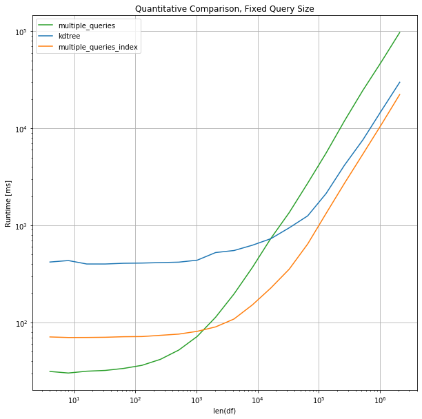
For this information range, the comparison betwixt kdtree, multiple_queries and the indexed version of multiple queries shows the expected behavior: The initial overhead of constructing the tree or the sorting of the data overweighs when searching confronting larger datasets. The kdtree is expected to outperform the indexed version of multiple queries for larger datasets.

It is to emphasize that as the scipy implementation easily accepts due north-dimensional data it is very straightforward to extend for even more dimensions.

Summary

Testing filtering speed for different approaches highlights how lawmaking can be effectively optimized. Execution times range from more than than 70 ms for a tiresome implementation to approx. 300 µs for an optimized version using boolean indexing, displaying more than 200x improvement. The principal findings can exist summarized as follows:

• Pure Python can exist fast.
• Numba is very benign even for non-optimized loops.
• Pandas onboard functions tin can exist faster than pure Python but likewise take the potential for improvement.
• When performing large queries on large datasets sorting the data is beneficial.
• g-d-trees provide an efficient style to filter in n-dimensional infinite when having large queries.

Execution times could be further speed upward when thinking of parallelization, either on CPU or GPU. Annotation that the retentiveness footprint of the approaches was non considered for these examples. When having files that are too big to load in retention, chunking the data or generator expressions can be handy. If you find that any approach is missing or potentially provides better results let me know. I am curious to run into what other means exist to perform fast filtering.

greenningdom.blogspot.com

Source: https://towardsdatascience.com/speeding-up-python-code-fast-filtering-and-slow-loops-8e11a09a9c2f

Share this post